
Conditional formatting in Excel - how it works
Related Videos: Excel: Conditional Formatting (May 2024).
In Excel, you can use conditional formatting to reshape the cell contents as you like. For example, you can display completely different text or change the font. The powerful toolset includes numerous options as well as predefined rules. This article shows the main types of rules for conditional formatting.
Conditional formatting: Format all cells based on their values
This type of Excel rule has graphical options, for example to visually decorate numerical values. This makes it easier for you to get an overview of your data.
- Select an area in the Excel spreadsheet and click on the "Start" tab.
- Now select "Conditional Formatting" and then click on "New Rule ...".
- In the new window, select the type "Format all cells based on their values".
Color-code cells using conditional formatting
You can easily find values that do not fall within a certain range with Excel. This function is used to color-code all cells whose content does not correspond to the value range.
- Select an area in the Excel spreadsheet and click on the "Start" tab.
- Go to "Conditional Formatting" and then to "New Rule ...".
- If you select "Classic", you configure that the cells that fall below or exceed a value are color-coded.
Conditional formatting: 2- and 3-color scale
You can add expression to the meaning of your values using a gradient. For example, on a scale from one to ten, show how much radiation is in an area.
- In the lower area of the window, select the "2-color scale" format style.
- As the type, select "Minimum" for minimum and "Highest" for maximum.
- If necessary, change the predefined colors and finish with "OK".
- For a 3-color scale you determine the formatting for the mean.

Conditional formatting in Excel: bars
You can also use bars for formatting. For example, graph your expenses per month in Excel.
- Simply select "Data Bar" as the format style.
- Select "Automatic" for the minimum and maximum.
- Design the representation of the bars below and conclude with "OK".

Symbol sets in conditional formatting
With the symbol sets you can, for example, enter the signal strength of a network in percent and use the appropriate symbols as a graphic means.
- Select the "Symbol sets" format style in the lower area of the window.
- Now select the display of the signal strength as the symbol type.
- With the first option "if value:" set this to ">". You can leave the rest like this. The Excel rule is completed with a click on "OK".

Conditionally format cells that contain a certain value
This format type is particularly suitable for highlighting individual special values. For example, all numbers under 0 can be marked with the color red.
- Select the area in the table that you want the formatting to apply to and create a new rule of the type "Format only cells that contain".
- Set the following option: "Cell value less than 0".
- Click on the "Format ..." button and select, for example, the color red in the new window.
- Click OK twice to create the rule

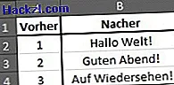
Conditional formatting: represent numbers as text
If you have predefined texts that appear again and again, this type is suitable. This not only saves you time, but also prevents typing errors.
- Select the area in the Excel spreadsheet to apply the formatting to and create a new rule of the type "Format only cells that contain".
- Use the following option: "Cell value equals 1"
- Click the "Format ..." button and select the "Numbers" tab in the new window.
- Click "Custom" in the left sidebar.
- In the text field under the label "Type:" enter the following: "Hello world!" - the quotation marks are mandatory.
- Click "OK" twice to complete the process.
- If you now enter the number one in a cell in your defined area, the text "Hello World!" Appears instead. You can define further texts for other numbers in exactly the same way.
Formula for determining the cells to be formatted
As the title suggests, this type reformats any value to which a particular formula applies. In this example, all Excel data that is still in the future is marked in red.
- Select the area of the table for which the formatting should apply and create a new rule with the type "Use formula to determine the cells to be formatted".
- Enter the formula = B2> TODAY ().
- Click on the "Format ..." button and select red as the color in the new window.
- Confirm the whole thing by clicking "OK" twice.

This article shows only a few uses of conditional formatting. The function can be used extremely versatile and with a little routine you can already achieve great results. These instructions refer to Excel 2010. In addition to the conditional formatting, Excel offers other useful functions.