
Link Excel files together - so it'll work
If you need the same data in different Excel files, linking the corresponding tables together is a good and, above all, time-saving solution. You can use Excel to link the different worksheets of a workbook as well as the tables from different workbooks.
Connect different office files in Excel
By connecting the tables, you ensure that you always have absolutely identical numbers in all linked cells. If you correct numbers in the original table, the corrections are automatically applied by the linked tables. In our small example, a company has several branches in different cities and we link the data from the "Sales per branch" worksheet with the "Sales per city" worksheet. You can of course enter the cell addresses to be connected manually, but the following variant is more practical:
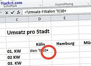
- We start with the table "Revenue per city", into which the daily revenues of all branches are to be transferred per city. To do this, go to cell D5, which after the link should contain the total sales of Cologne in the first calendar week.
- Enter an equal sign in cell D5 and then go to the "Sales per branch" worksheet, which contains the data to be linked.
- There, click on cell E10, in which the total sales of all Cologne branches from 02/01/2014 are and then press the [Return] key.
- You will then automatically be back on the "Revenue per city" worksheet. The previously selected cell D5 now contains the same data as cell E10 in the "Sales per branch" worksheet.
- If you now change any number in the "Sales per branch" table belonging to cell E10, the number in cell D5 in the "Sales per city" worksheet is also automatically changed.
Arithmetic operations with linked Excel cells
- Of course, you can also perform arithmetic operations with the linked cells in Excel.
- In our small example, we add in the linked cell D5 of the table "Sales per city" all daily sales of the first calendar week from the table "Sales per branch". The worksheet "Revenue per city" in cell D5 finally contains the total revenue from Cologne for the first week of 2014.
- To achieve this, first go to cell D5 in the "Revenue per city" table and add a plus sign to the link.
- Then go to cell F11 in the "Sales per branch" worksheet, which contains Cologne's total sales for 03/01/2014.
- If you close the link with the [Return] key, you are back on the "Sales per city" worksheet and the amount in cell D5 is now made up of the sum of two daily sales.
- Of course, you can also manually enter the missing days of the calendar week in the formula. You just add the appropriate cells to the "Revenue per store" table.
- In our example, it looks like this: = 'Sales branches'! E10 + 'Sales branches'! F10 + 'Sales branches'! G10
If you have formatted your tables and want to prevent the formatting from being accidentally removed, we will show you how it's done here.
Latest videos
We type equal signs in cell D5 to be linked in the table "Revenue per city".

In the "Sales per branch" table, we select the cell E10 to be linked.

After the link, both tables get the same number.

In cell D5, we add a plus sign to the formula to add up the daily sales.
We link the next daily turnover from the table "turnover per branch" - cell F10 - with cell D5 in the table "turnover per city".
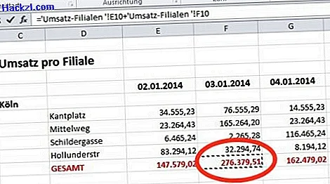
The amount in cell D5 now includes two daily sales.
