
Excel: Mark negative numbers red & positive green
In Excel you can mark negative numbers in red and positive numbers in green so that you always have an overview, even in larger tables. Our instructions show you how to do this in just a few steps.
Mark negative numbers in red in Excel
- First mark all cells in Excel that you want to color red or green. If the cells are widely scattered, you can also select them individually while holding down the [Ctrl] key.
- Then right-click in one of the markings to open the context menu.
- Here you select the "Format cells" option.
- In the upper ribbon click on "Numbers" and then at the bottom on the entry "User-defined":
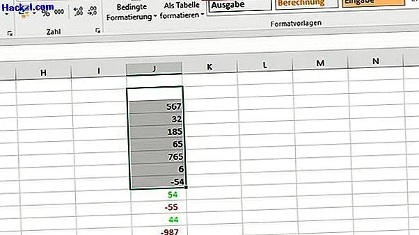
- Insert the following into the input field: [Green] #. ## 0 _ €; [Red] - #. ## 0 _ €
- If you click on "OK", all negative numbers are colored red and all positive numbers green.
- To do this, click on the relevant cell or select several cells.
- Now select the large button "Standard" in the "Format" section of the "Start" menu at the top.
- The selected cells then appear in the standard design with black letters.
Next we will show you on the next page how to embed images in Excel.