Excel: create ranking lists automatically
By creating ranking lists, individual values can be sorted in Excel. Our instructions show you how to do this.
Step 1: prepare ranking in Excel
In this example we show how to do it:
- We write down our values in cells A2 to A10. The ranking list should appear in cells B2 to B10.
- Note: The "RANK.GLEICH" function is used to create the ranking list. In older versions of Excel this is only "RANG".

Step 2: Create ranking list automatically in Excel
- Click with the mouse in the cell in which the ranking starts. In this example B2.
- Switch to the "Formulas" tab above and click on the "Insert function" button.
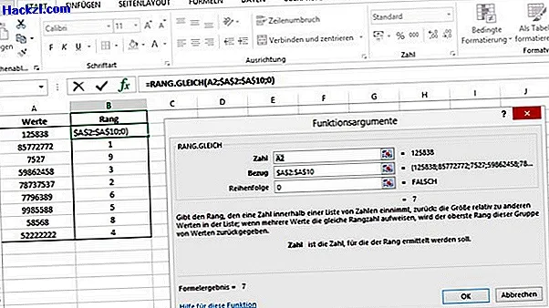
- Select "Statistics" as the category and "RANK.EQUAL" as the function. Confirm the process with "OK", a new window opens.
- Click in the "Number" field and then select the top cell of the values. In this case A2.
- In the "Reference" field, mark the area between the first and last value. Here A2: A10.
- If you press the [F4] key, the cover is automatically converted into the appropriate format. So A2: 10 becomes $ A $ 2: $ A $ 10.
- If you enter 0 (zero) in the Order field, the highest value is ranked 1. If you enter a 1 instead of 0, the lowest value is ranked 1.
- If you close the window with the "OK" button, the first rank appears. If you simply drag the cell down, the complete ranking is created.