
Excel: Show and hide columns faster
To print your Excel spreadsheets, hide individual columns or rows and then later to edit them again. So far, you have painstakingly switched all columns individually. However, you can save yourself these repeated steps.
Arrange Excel columns and rows in an outline
Work with outlines - you can use them in Excel similar to the function of the same name in Word. If you arrange the relevant columns or rows on different outline levels, you can do the annoying hiding and showing of individual areas with a click of the mouse. Here's how:
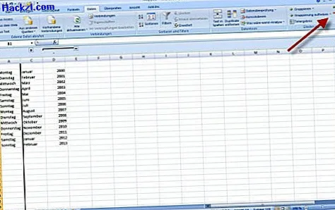
- Select a column to be hidden. Then open "Data | Grouping and Outlining | Grouping" or in Excel 2007 "Data | Group | Grouping".
- Excel downgrades the marked areas to the second structuring level and displays an additional header at the top that shows the individual levels.
- The columns will initially continue to be displayed. Repeat the process for the remaining columns that you want to hide. Related markings can be downgraded together.
- To hide the areas formatted in this way, all you need to do is click on the small symbol "1" on the left in the outline header. With a click on "2" you will later show the second structure level again.
- Individual columns can also be easily displayed: To do this, click on the plus sign above the adjacent column.
Note:
Marked areas can be moved to the next lower level by repeatedly using the outline function. Excel offers a total of eight levels. If you are bothered by the outline display, you can quickly hide the line with the key combination [Ctrl] + [7] and show it again later. This structuring principle works in the same way for rows.