
Creating a pivot table in Excel: a quick start guide
The creation of pivot tables in Excel is ideal for larger amounts of data that should be clearly displayed and evaluated. With this practical tip, you can create a pivot table with Microsoft Excel 2010 in just a few steps.
Selection of the Excel data area
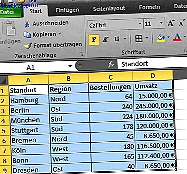
In principle, several tasks and evaluations can be solved in parallel with pivot tables. In our example we would like to determine the number of orders as well as the turnover of the region "South". To prepare your data for use in a pivot table, you must first select the relevant data area.
- To do this, click in the first cell of your Excel worksheet, hold down the right mouse button and mark the desired area. This area should now be marked "blue".
Creation of the pivot table
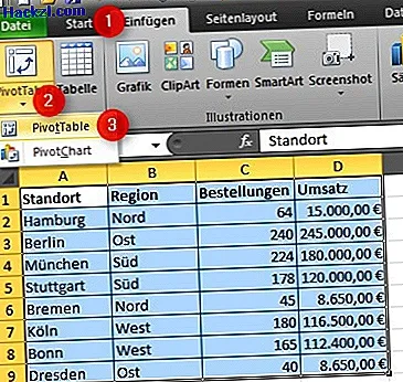
- Now click on the "Insert" tab. In the overview, the symbol for the "pivot table" wizard appears, which you now click with the left mouse button.
- Then the wizard opens, which will help you with the further creation. Based on the selection of your data area in the first section, the options "Select table or area" and table / area "are already pre-assigned. Excel offers further functions, such as the use of an external data source (e.g. Access database or SQL server), but we won't go into that here.
- The data area is selected - now you have to determine whether your pivot table should be created in a new or in the existing worksheet. For our example we use the "New worksheet" option. The base of the pivot table is now created.
Adjustment of the pivot table
The next step to your finished pivot table is to adjust the values. This is possible via the "pivot table field list", which should now be displayed. In the upper area of the field list you will find the data fields from your selected data area. In the lower part you can define "Report filter", "Column and row labels" and "Values". As mentioned at the beginning, we would like to determine the number of orders as well as the turnover of the region "South". The following adjustment is necessary:
- Drag the Region field to the Report Filters area. This is necessary in order to carry out filtering on the "South" region.
- Drag the Location field to the Row Labels area.
- Finally, drag the "Orders" and "Sales" fields into the "Values" field.

Finishing touches - The finished pivot table
After you have placed all the data fields in the pivot table, you can close the field list. It can be shown again at any time from the table by clicking the right mouse button.
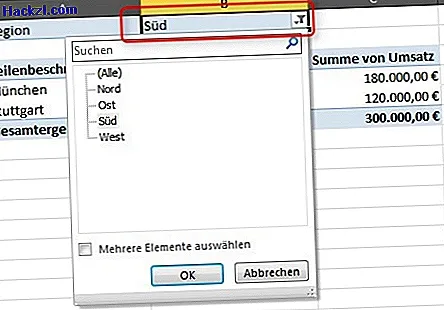
- Finally, adjust the filter of the "Region" field by clicking on the filter symbol and selecting the value "South". The table is now created and can be used.
Become an Excel professional with the new course at the CHIP Academy
With the course in the CHIP Academy "Excel: Pivot tables in less than an hour" even beginners learn how to handle a large amount of data quickly and easily.
- Learn in 40 minutes from our lecturer Daniel Kogan what pivot tables are and how to use them sensibly.
- You will learn how to use pivot tables and pivot charts to gain insights and insights from your data that you would otherwise not have been able to access.
- Visit the CHIP Academy and get the extensive online video workshop for 19.90 euros.
Microsoft Windows 7 SP1, Microsoft Excel 2010.