
Lock or protect cells in Excel
If you lock individual cells in Excel, they can no longer be changed, but the remaining rows and columns of the workbook can. In this tip, we show how to apply this protection.
Lock cell in Excel - the preparation
Protecting one or a few cells is a bit more cumbersome than locking an entire worksheet:
- First of all click with the right mouse button on the small gray square, which you will find in the top left between the column name and the row numbering.
- The entire work area is now colored blue and the context menu is open.
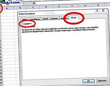
- In the context menu, select "Format cell" and select the "Protection" tab
- The "Locked" option is activated by default, you deactivate the function and exit the menu by clicking "OK".
- Now select the cell or cells you want to lock.
- If there are several cells that are not next to each other, click on the cells individually while holding down the [Ctrl] key.
- Then right-click to open the context menu again and click on "Locked" in the "Protect" tab.
Protect Excel cells reliably - step 2
You now have two options for activating the cell protection function.
- You could select the "Protect Sheet" icon in the quick start bar from the "Review" tab.
- Or you can opt for the much faster route and right-click on the corresponding tab in the lower sheet area.
- Then select "Protect sheet" in the context menu.
- If you want, assign a password for your cells in the "Protect sheet" menu or confirm immediately with "OK".

If you have given your worksheet a password and forgotten it, we will tell you here how you can access the workbook again.